Pandas is a powerful Python library for working with structured financial data. It provides intuitive data structures—like Series (for single columns of data) and DataFrames (for full tables)—that make it easy to clean, analyze, and transform datasets such as price histories, income statements, trading logs, or economic indicators.
In financial workflows, Pandas is used for a wide range of tasks: loading time series data (e.g., stock prices), calculating returns and volatility, aggregating trades by day or asset, building factor models, and cleaning large sets of transaction data. Analysts use it to automate reporting, build dashboards, backtest trading strategies, and prepare data for statistical modeling or machine learning. It’s particularly well-suited to working with time-indexed data and integrating multiple sources—such as Bloomberg exports, market data feeds, or financial statements.
What makes Pandas so valuable in finance is its ability to handle real-world data: it deals gracefully with missing entries, irregular timestamps, and mixed data types—all common challenges in financial analysis. Whether you’re managing a hedge fund model, analyzing bank performance, or building an earnings forecast, Pandas helps you turn raw financial data into clear, actionable insights.
In this guide, we’ll walk through the basics of getting started with Pandas — from loading and exploring data in your first dataframe, to mid-level topics like grouping, merging, reshaping, and working with time series. Whether you’re a beginner looking to understand the fundamentals or an intermediate user aiming to deepen your skills, this article is designed to be your practical companion in learning how to think—and code—with Pandas.

Pandas gives you a powerful, Python-based toolkit for working with structured data.
It’s a library that allows you to load data from external sources like CSVs, Excel, SQL databases, or APIs, then quickly explore, clean, and transform it. With just a few lines of code, you can filter transactions, calculate financial metrics like returns or profit margins, and organize your data into meaningful groups, such as revenue by region or cost per product.
Once your data is structured, Pandas helps you analyze and summarize it. You can sort, rank, and reshape datasets, apply custom functions, or build pivot tables to get deeper insights. Its grouping and aggregation tools make it easy to compute KPIs across time periods, client segments, or asset classes. For financial time series, Pandas offers built-in support for datetime indexing, resampling, and rolling statistics, enabling accurate modeling and historical analysis.
Pandas also integrates seamlessly with other libraries like Matplotlib for quick visualizations, and scikit-learn for machine learning workflows. Whether you’re preparing an earnings report, building a forecasting model, or analyzing trades, Pandas lets you move from raw data to insight efficiently—making it an essential tool for modern financial analysis.
To use Pandas effectively, you need to first understand its two fundamental building blocks: Series and DataFrames.
A Series is like a single column of labeled data. You can think of it as a list with names attached—each value has an associated label called an index. This makes it easy to refer to values not just by position, but by a meaningful key (like a date, a stock ticker, or a customer ID). Series are great for 1D data—like a time series of prices or a list of countries with population counts.
A DataFrame is a table made of multiple Series. Each column is its own Series, and all the columns are aligned by their index (row labels). This two-dimensional structure is what makes Pandas so powerful for real-world datasets. DataFrames let you work with full tables of information—like balance sheets, trading logs, or multi-column reports—while preserving the relationships between variables.

Creating a series in Pandas is as simple as calling the Series() constructor function.
To do that; importing pandas, declaring an array of data, and its corresponding indices.
     import pandas as pd

s = pd.Series([100, 200, 300], index=['AAPL', 'MSFT', 'GOOG'])

print(s)
Calling print(s) results in the following series being printed to the output area.
     AAPL    100
MSFT    200
GOOG    300
dtype: int64
Here’s what’s happening conceptually:
pd.Series refers to the Series class or constructor function from the Pandas library.
When you write pd.Series(...), you are creating a new Series object by calling that constructor and passing it:
A list of values: [100, 200, 300]
An index (labels for each value): ['AAPL', 'MSFT', 'GOOG']

     data = {
    'Company': ['AAPL', 'MSFT', 'GOOG'],
    'Price': [100, 200, 300],
    'Sector': ['Tech', 'Tech', 'Tech']
}

df = pd.DataFrame(data)
print(df)
       Company  Price Sector
0    AAPL    100   Tech
1    MSFT    200   Tech
2    GOOG    300   Tech
One of the most powerful features of Pandas is the ability to create a DataFrame out of a variety of very common formats that financial data comes in.
You can create a DataFrame from:
A dictionary of lists or Series (most common), or list of dictionaries
A CSV, Excel, SQL, or JSON file
A NumPy array
Take, for example, the process of turning a CSV file into a DataFrame for analysis in Pandas.
df = pd.read_csv('stocks.csv')
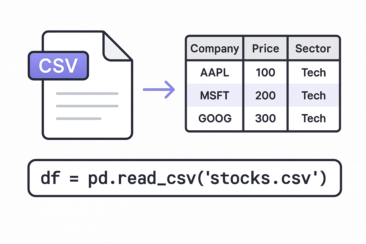
Yes! It’s that simple.
Pandas will read your CSV, and translate your Excel into an indexed group of series, ready to perform data analysis on.
Pandas also supports many other formats. For example, MySQL (as well as SQL operations) are fully supported, which allows analysts to create and take slices of larger datasets, and shape a dataframe from a larger database.
     import sqlite3
conn = sqlite3.connect('mydb.sqlite')
df = pd.read_sql_query("SELECT * FROM stocks", conn)
We’ve imported our CSV, and we have our first DataFrame – now what? Our first step in working with dataframes is to understand the most common “worker-functions” that will allow us to quickly explore, gut-check, and understand our data as we are working with it.
Here are several common functions, in no particular order:
| Function | Purpose |
|---|---|
.head(n) | View first n rows |
.tail(n) | View last n rows |
.info() | Summary of types, nulls, and memory usage |
.describe() | Descriptive statistics for numeric columns |
.shape | Get (rows, columns) |


Now that you understand the two core data structures in Pandas—Series and DataFrames—it’s time to get practical. This section walks you through the most common operations you’ll perform when working with data in Pandas: loading data, inspecting it, filtering it, transforming it, and preparing it for analysis.
One of the most common first tasks you’ll need to do in Pandas is to take a DataFrame and select (or filter) your data based on a set of criteria.
Boolean indexing in Pandas allows you to filter rows in a DataFrame based on a condition that returns either True or False. It is one of the most intuitive and commonly used ways to slice a dataset. For example, you might want to isolate all transactions over $1 million, or all deals in the ‘Healthcare’ sector. You simply pass a condition inside square brackets—such as df[df[‘Revenue’] > 1_000_000]—and Pandas returns only the rows where the condition is true. This method is highly useful in finance for quickly analyzing outliers, thresholds, or any data that meets certain performance or classification criteria.

     df['Revenue']            # Single column (as Series)
df[['Revenue', 'Cost']]  # Multiple columns (as DataFrame)
You can filter rows by boolean operators. (or even functions!)

     df[df['Revenue'] > 1000]         # Only rows with Revenue > 1000
df[df['Region'] == 'West']       # Only rows where Region is 'West'

df[(df['Revenue'] > 1000) & (df['Region'] == 'West')]
An alternative to filtering a DataFrame by boolean indexing: Pandas offers the ability to filter data by integer based index or label based indexing.
.iloc[] — Integer-position indexingIn a DataFrame, all rows have a numeric index. .iloc[] allows you to access rows by this integer-based index. Starting with the first row as row 0. iloc[] accepts a single integer, a list of integers, or a slice of integers. It allows you to select rows and columns by their integer positions in the DataFrame, which is especially helpful when you’re working with data whose column names aren’t known ahead of time or when you’re dealing with time slices.
For instance, if you want to get the first five rows and the second and third columns, you would use df.iloc[0:5, [1, 2]]. In finance, .iloc[] can be helpful for tasks like extracting the last 4 quarters of revenue or the first 10 rows in a screening model output, where the row or column positions are predictable and consistent.
For advanced filtering, .iloc[] can also accept arrays and single variable functions.
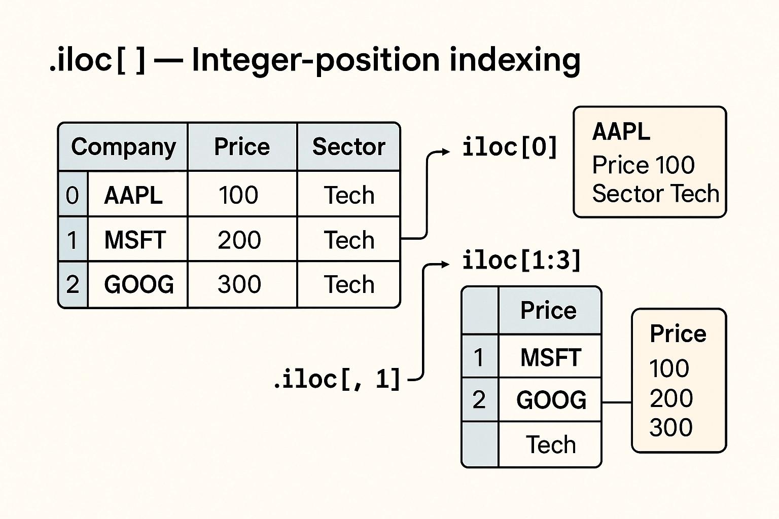
     df.iloc[0]      # First row
df.iloc[1:3]    # Rows 1 and 2
df.iloc[:, 1]   # All rows, second column
.loc[] — Label-based indexingAlternatively, Pandas also allows you to access a group of rows and columns by its label(s) using .loc[].
The .loc[] method is used for label-based indexing, letting you select data by row and column names. It’s more descriptive and flexible than boolean indexing or .iloc[], especially when you need to select specific columns based on a condition.
For example, df.loc[df[‘Region’] == ‘EMEA’, [‘Company’, ‘Revenue’]] would return just the Company and Revenue columns for companies in the EMEA region. It also works well with datetime indexes—like selecting data between two dates—and is often used in financial applications where you’re working with named fields such as ‘EBITDA’, ‘Revenue’, or ‘Close Price’.
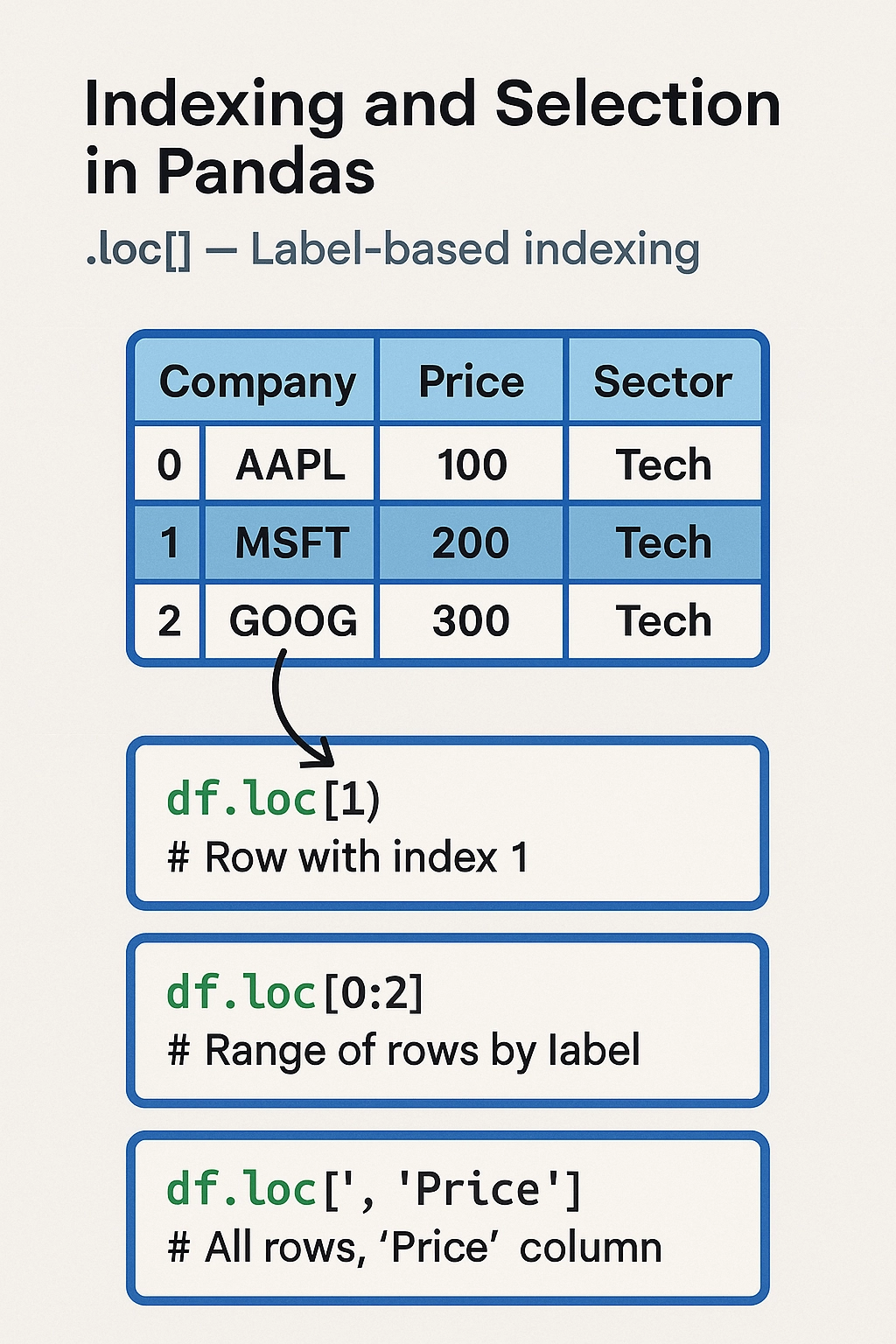
     df.loc[1]       # Row with index 1
df.loc[0:2]     # Range of rows by label
df.loc[:, 'Price']  # All rows, 'Price' column
Once you have selected and filtered the data in a DataFrame, you can begin with basic manipulations, such as sorting and ranking.
In finance, sorting and ranking are essential tools for prioritizing and analyzing data within a DataFrame. Sorting allows you to reorder your dataset based on values in one or more columns—such as sorting a list of deals by deal size (df.sort_values(‘Deal Size’, ascending=False)) or sorting securities by return. Ranking, on the other hand, assigns a relative position to each row based on a specific metric. For example, you might use df[‘Return Rank’] = df[‘Return’].rank(ascending=False) to identify top-performing assets in a portfolio. This is particularly useful in investment banking and private equity for tasks like identifying the top 10 M&A deals, ranking companies by EBITDA multiples, or preparing league tables. Combined with filtering and aggregation, sorting and ranking turn raw data into actionable insights.

     df.sort_values(by='Revenue', ascending=False)   # Sort by column
df.sort_values(by=['Region', 'Revenue'])        # Multi-column sort
df['Rank'] = df['Revenue'].rank(ascending=False) # Add a rank column
Pandas makes it easy to pivot, melt, and reshape data from wide to long formats and back.
In finance, reshaping data with pivot and melt is incredibly useful when transforming data between different analytical views. The pivot() method helps convert data from a long format to a wide format—for instance, turning a transaction log into a table where each row is a company and each column is a fiscal quarter with corresponding revenue values. This makes it easier to perform time-series analysis or generate management reports. On the other hand, melt() (also known as unpivoting) is used to convert wide-format data back into long format, which is ideal for running grouped operations, plotting, or exporting to systems that expect tidy data.
For example, in private equity, a pivot table might help an analyst compare EBITDA margins across portfolio companies by quarter. Later, melting the data could help reformat it for regression analysis or visualization. These reshaping operations streamline the workflow when toggling between analysis-ready and presentation-ready data structures.
Pivoting in Pandas refers to transforming or reshaping a DataFrame from a long format to a wide format. It’s a powerful way to reorganize your data so that columns become rows, or vice versa, depending on your analysis needs.
Conceptually:
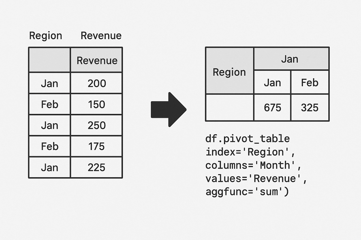
df.pivot_table(index='Region', columns='Month', values='Revenue', aggfunc='sum')

pd.melt(df, id_vars='Region', value_vars=['Jan', 'Feb', 'Mar'])
.apply() to run custom functionsUsing .apply() in Pandas allows you to run a custom function across a DataFrame or Series — row-wise or column-wise. When used on a Series, .apply() applies a function to each element. When used on a DataFrame, you specify whether to apply the function row-wise (axis=1) or column-wise (axis=0).
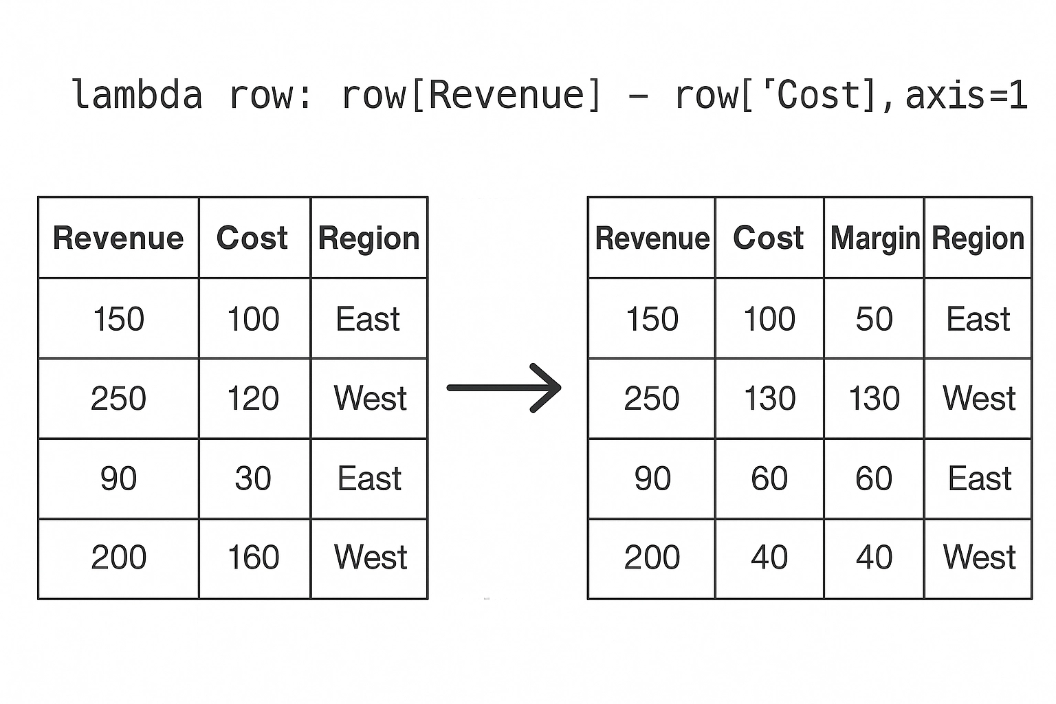
df['Margin'] = df.apply(lambda row: row['Revenue'] - row['Cost'], axis=1)
.map() on a Series
df['Region_Code'] = df['Region'].map({'West': 1, 'East': 2, 'North': 3})
Before you can analyze or model your data, often times you need to clean it. This step is often where data scientists spend most of their time — and Pandas makes it significantly easier with a rich set of tools for wrangling messy, inconsistent, or incomplete data.
This section covers the most common data cleaning and preprocessing techniques in Pandas.
Missing data is a common issue during financial modeling, valuation, or due diligence—especially when aggregating data from multiple sources like company financial statements, data rooms, or market databases. Pandas has a number of very useful helper functions to identify, remove, and correct missing data in datasets.
Detecting missing data is an essential part of data cleaning in Pandas. It allows you to identify and handle gaps in your dataset, such as blank cells, NaN values, or missing timestamps.

     df.isna()             # True/False for each cell
df.isnull().sum()     # Count of nulls per column
Removing missing data in Pandas is a crucial step when preparing your dataset for analysis or modeling. The df.dropna() method helps eliminate rows or columns that contain NaN (missing) values, giving you control over how clean your data needs to be.

     df.dropna()                   # Drop any rows with NaNs
df.dropna(axis=1)            # Drop columns with any NaNs
df.dropna(subset=['Price'])  # Drop rows where 'Price' is NaN
Filling missing data in Pandas is a flexible and powerful way to handle NaN values without discarding valuable rows or columns. The .fillna() method lets you replace missing values using a variety of strategies depending on the context of your dataset.
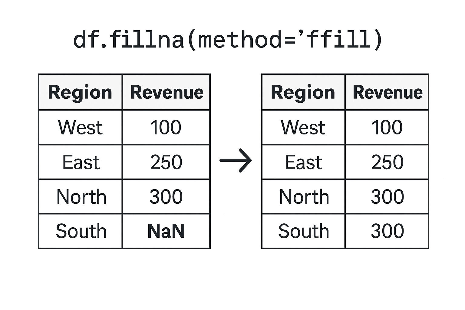
     df.fillna(0)                         # Replace NaNs with 0
df.fillna(method='ffill')           # Forward fill (use previous value)
df.fillna(df['Revenue'].mean())     # Replace with column mean
Duplicate rows can skew results, especially in aggregations. Pandas’ df.duplicated() identifies rows that are duplicates of previous ones by returning True for each repeated row, while df.drop_duplicates(inplace=True) permanently removes those duplicate rows from the DataFrame, keeping only the first occurrence.

     df.duplicated()                 # Returns True for duplicated rows
df.drop_duplicates(inplace=True)  # Removes duplicated rows
You can also drop based on specific columns:
df.drop_duplicates(subset=['CustomerID', 'OrderID'])
You can clean inconsistent formatting or standardize values:

     df['Status'].replace({'pending': 'Pending', 'PENDING': 'Pending'}, inplace=True)
df['Category'].replace('Misc', np.nan, inplace=True)  # Convert to NaN
Pandas automatically infers data types, but you often need to correct or convert them.

     df['Date'] = pd.to_datetime(df['Date'])        # Convert to datetime
df['Price'] = df['Price'].astype(float)        # Convert to float
df['Region'] = df['Region'].astype('category') # Convert to categorical type
Use .dtypes to check current types and .astype() for manual changes.
Text data often needs normalization (especially when imported from spreadsheets or manual entry):
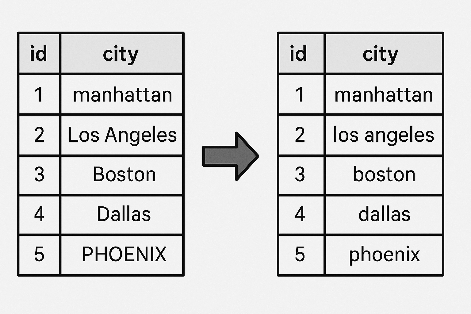
     df['city'] = df['city'].str.strip().str.lower()
df['product'] = df['product'].str.replace('-', ' ').str.title()
Use .apply() to run a function across rows or columns:

     def categorize(row):
    if row['Revenue'] > 1000:
        return 'High'
    else:
        return 'Low'

df['Revenue_Level'] = df.apply(categorize, axis=1)
One of the amazing features of the DataFrame is the ability to create new columns from existing data; either from

     df['Profit'] = df['Revenue'] - df['Cost']
df['Revenue_per_Item'] = df['Revenue'] / df['Quantity']
df['Is_High_Value'] = df['Revenue'] > 500

     df.rename(columns={'Rev': 'Revenue'}, inplace=True)
df.columns = df.columns.str.lower()  # Make all columns lowercase
Once your data is clean and structured, you’ll often want to summarize it — to calculate totals, averages, counts, or other metrics across categories or time periods. That’s where Pandas’ powerful groupby functionality comes in.
This section walks you through grouping, aggregating, and summarizing data using real-world patterns.
The groupby() method follows a simple, powerful pattern:
Split → Apply → Combine
You split the data into groups based on some key(s), apply a function to each group independently, and then combine the results into a new DataFrame or Series.


df.groupby('Region')['Revenue'].sum()
Want the average revenue instead?

df.groupby('Region')['Revenue'].mean()
Want multiple aggregations?
df.groupby('Region')['Revenue'].agg(['sum', 'mean', 'max'])
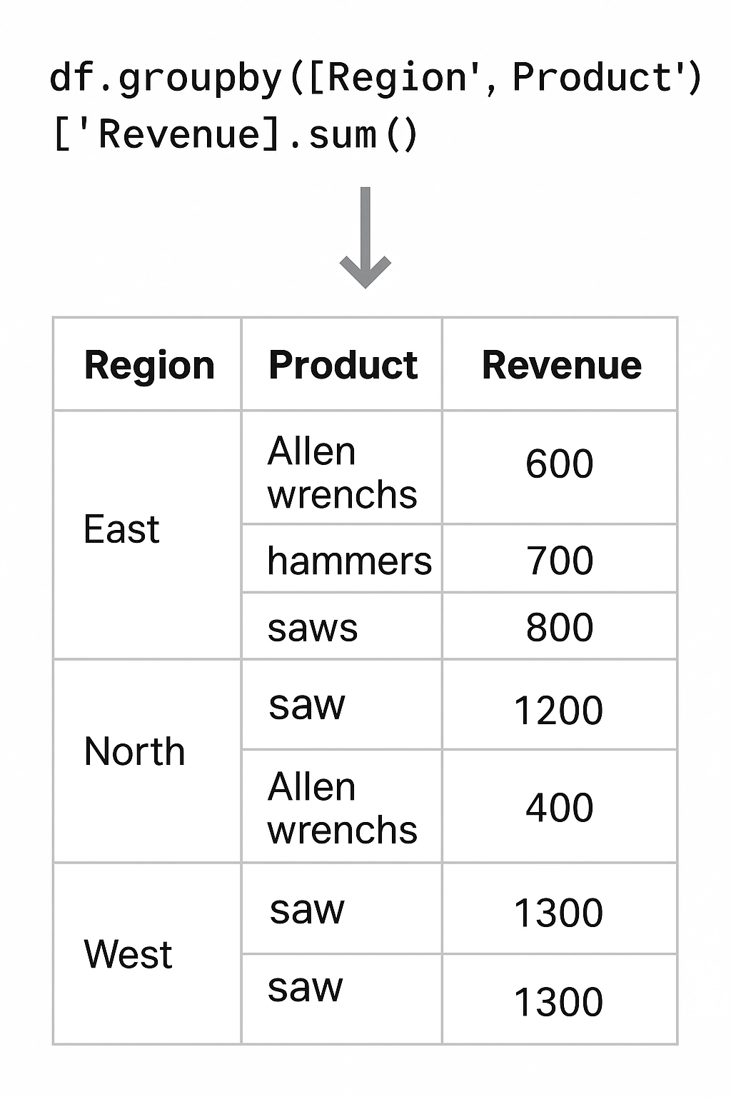
You can group by more than one column to get hierarchical summaries.
df.groupby(['Region', 'Product'])['Revenue'].sum()
This returns a MultiIndex result — a layered index that lets you drill down into combinations of dimensions.
After grouping, your index becomes the grouping column(s). You can convert it back to regular columns using .reset_index():

grouped = df.groupby('Region')['Revenue'].sum().reset_index()
This is especially helpful for exporting or plotting.
You can use .filter() to return only those groups that meet a condition.
Example: keep only regions with more than 100 total orders:
df.groupby('Region').filter(lambda x: x['OrderID'].count() > 100)
agg()The .agg() method lets you apply multiple functions at once, or use custom ones.
     df.groupby('Region').agg({
    'Revenue': 'sum',
    'Cost': 'mean',
    'OrderID': 'count'
})
You can also define your own functions:
df.groupby('Product')['Revenue'].agg(lambda x: x.max() - x.min())
When grouping by multiple columns, Pandas returns a MultiIndex object, which can be flattened if needed:
     grouped = df.groupby(['Region', 'Product'])['Revenue'].sum()
grouped = grouped.unstack()   # Makes 'Product' columns, 'Region' rows
df.groupby('Region')['Revenue'].describe()
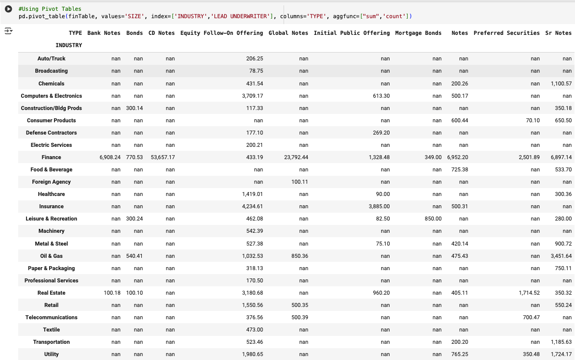
Pivot tables provide a cleaner syntax for grouped summaries, especially in 2D.
Pivot tables provide a cleaner syntax for grouped summaries, especially in 2D.
df.pivot_table(index='Region', columns='Month', values='Revenue', aggfunc='sum')
In real-world projects, your data rarely lives in a single file or table. Instead, you’ll often work with multiple datasets that need to be combined—for example, transactions with customer info, or products with pricing tables.
Pandas offers powerful tools for merging and joining, inspired by SQL but made even more flexible.
The merge() function is the most common function for combining data, and is used to join DataFrames together based on one or more common keys.
To understand the merge() function – the best resource is to start by becoming comfortable with SQL joins. Below is a brief overview of the four common types of joins, and how each leads to very different data in your post-join dataframe.
By default, when you use the .merge() function – Pandas will assume you are attempting an Inner Join on your data.
In this case, only rows where your key exists in both DataFrames will be included in your resulting DataFrame. Rows with unmatched keys will be removed from your resulting DataFrame.

     pd.merge(customers, orders, on='CustomerID') #Default merge - assumes inner join
pd.merge(df1, df2, on='ID', how='inner')  # Explicit inner join
Keeps all rows from df1, the left DataFrame.
Use when: You want to preserve everything from df1 and only add data from df2 where available.
pd.merge(df1, df2, on='ID', how='left') # Left join
Keeps all rows from df1, the left DataFrame.
Use when: You want to preserve everything from df1 and only add data from df2 where available.
pd.merge(df1, df2, on='ID', how='right') # Right join
Keeps all rows from both df1 and df2.
Use when: You want a complete view, including all unmatched records from both sides.
pd.merge(df1, df2, on='ID', how='outer') # Full outer join
join()MethodIn addition to the merge() function, Pandas offers a DataFrame method join() for
DataFrame.join() is a convenient method when you’re joining on a single key or index. The Join() method is called on the left-hand dataframe.
df1.set_index('ID').join(df2.set_index('ID'))
You can also pass how='left', how='right', etc., just like merge().
concat()pd.concat() to stack DataFrames vertically or horizontally. 
pd.concat([df1, df2], axis=0)

pd.concat([df1, df2], axis=1)
Add ignore_index=True if you want to reset the index during vertical concatenation.
One of Pandas’ most powerful and underrated features is its built-in support for time series data.
This is incredibly important in Finance applications where the vast majority of data is time series. Whether you’re analyzing stock prices, forecasting sales, or aggregating sensor data by minute, Pandas provides the tools to work with time-based data intuitively and efficiently.
The first step to prepare your DataFrame for working with time series data is to convert your appropriate columns to datetime using pd.to_datetime():

df['Date'] = pd.to_datetime(df['Date'])
Once a column is in datetime format, you can:
Extract components (.dt.year, .dt.month, .dt.day)
Filter by date
Sort chronologically
Use it as an index for time-based operations
Setting a datetime column as the index unlocks time series functionality:
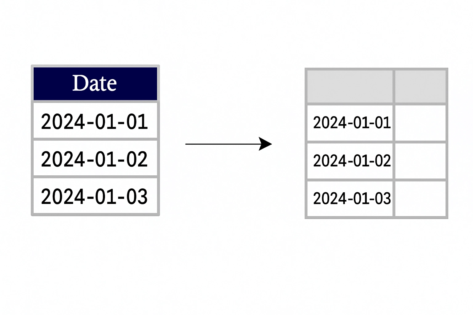
df = df.set_index('Date')
Now you can slice by date:

     df['2023']           # All data from 2023
df['2023-03']        # All data from March 2023
df['2023-03-15']     # Exact day
You can also sort by time:
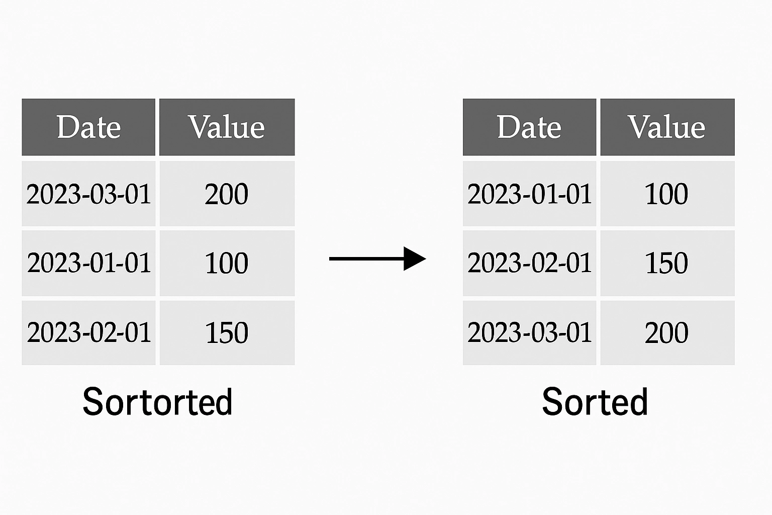
df = df.sort_index()
Resampling lets you convert between frequencies—e.g., from daily to monthly, or hourly to weekly.
     df.resample('M').mean()    # Monthly average
df.resample('Q').sum()     # Quarterly totals
| Code | Frequency |
|---|---|
'D' | Day |
'W' | Week |
'M' | Month-End |
'Q' | Quarter-End |
'Y' | Year-End |
'H' | Hour |
'T' or 'min' | Minute |
Rolling functions help you smooth out noisy time series data or compute metrics over a trailing window.
This calculates a 7-day moving average.

df['RollingAvg'] = df['Price'].rolling(window=7).mean()
You can also use .apply() with custom functions on rolling windows.
     df['RollingStd'] = df['Price'].rolling(30).std()
df['RollingMin'] = df['Price'].rolling(14).min()
df['Yesterday'] = df['Price'].shift(1)
This is useful when combining global datasets or aligning financial markets across time zones.
     df.index = df.index.tz_localize('UTC')               # Add time zone
df.index = df.index.tz_convert('America/New_York')   # Convert
Congratulations! You’ve made it to data visualization.
Data visualization is key to understanding trends, spotting anomalies, and communicating insights. While libraries like Matplotlib, Seaborn, and Plotly are great for custom plots, Pandas provides convenient built-in plotting methods that cover most day-to-day needs—especially for quick exploratory analysis.
These plotting tools are powered by Matplotlib under the hood, so you get the best of both worlds: fast prototyping and customizable output.
To use plotting in Pandas, you’ll first need to ensure Matplotlib is installed:
pip install matplotlib
When you call .plot() on a time series or numeric column, Pandas defaults to a line plot:
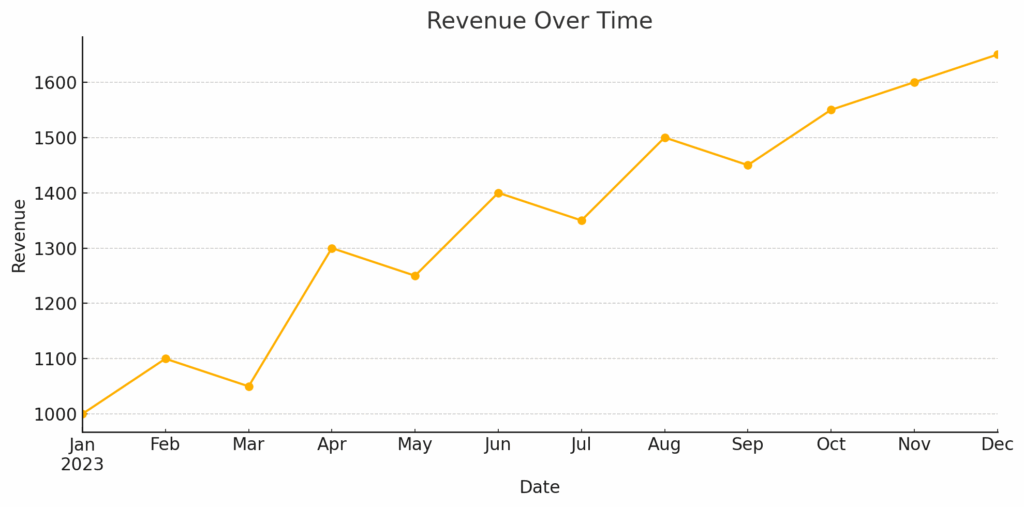
df['Revenue'].plot()(title='Revenue Over Time')
This is especially useful for:
Time series (daily prices, sales, etc.)
Trends over periods
Use bar plots to compare categories:

df.groupby('Region')['Revenue'].sum().plot(kind='bar', title='Revenue by Region')
Use kind='barh' for a horizontal bar chart.
Histograms help you understand the distribution of a single variable:
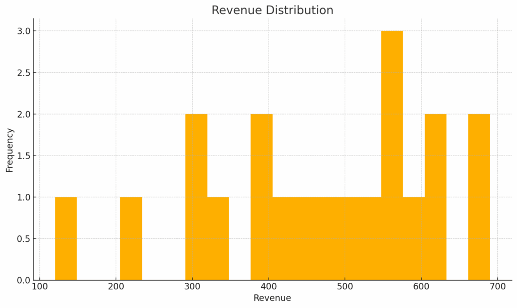
df['Revenue'].plot(kind='hist', bins=20, title='Revenue Distribution')
This is useful for spotting skewed data or outliers.
Boxplots show median, quartiles, and outliers—great for comparing distributions across groups:
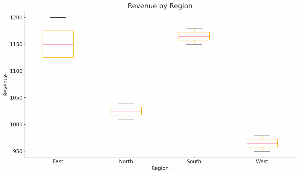
df.boxplot(column='Revenue', by='Region')
To show relationships between two numeric variables:
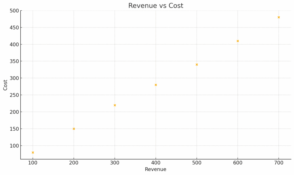
df.plot(kind='scatter', x='Revenue', y='Cost')
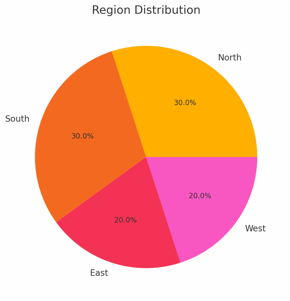
These are less common but available for completeness:

     df.plot(kind='area', stacked=False, alpha=0.4)
df['Region'].value_counts().plot(kind='pie', autopct='%1.1f%%')
These are less common but available for completeness:
     df.plot(kind='area', stacked=False, alpha=0.4)
df['Region'].value_counts().plot(kind='pie', autopct='%1.1f%%')
Since Pandas uses Matplotlib, you can customize your plots extensively:
     import matplotlib.pyplot as plt

ax = df['Revenue'].plot(title='Revenue Over Time', figsize=(10, 5), color='green')
ax.set_xlabel('Date')
ax.set_ylabel('Revenue ($)')
plt.grid(True)
plt.show()

df[['Revenue', 'Cost']].plot()
This produces a multi-line plot showing both series for easy comparison.
You can save any Matplotlib figure using:
plt.savefig('revenue_plot.png')
Learn the essentials of working with Pandas as part of our Python 1: Core Data Analysis Course: