Evaluating an Excel Formula with “Edit” Mode and the F9 Key

Almost everybody knows that pressing the F9 key in Excel recalculates all of the worksheets within all of the workbooks that a user has open. What many people don’t know, however, is that F9 can also be used to understand and debug formulas.

In Excel, there are typically many ways to perform the same task, so it should be no surprise that there are multiple ways to evaluate formulas.

The quickest way to evaluate a formula in Excel is to press CTRL + ~ (tilde). This toggles the display of the current worksheet, allowing you to switch views between cell values and cell formulas.  This is great for simply understanding how a formula works or for finding out the positioning of a #REF! error – especially over an area containing multiple cells.

If you require additional insight into how your formula or subset of your formula is working, you can evaluate the formula on a more granular level using Excel’s Evaluate Formula feature (Alt + M + V).  This allows you to evaluate the formula on a cell-by-cell basis.  However, there are two key limiting factors to this feature: (i) you can only evaluate the formula from left to right, and (ii) edits cannot be made directly within the Evaluate Formula dialog box.

To overcome these limitations, you can use the F9 key to evaluate your formula or a subset of your formula.  To do this, you must first press the F2 key on your desired cell to activate “Edit” mode (see our prior keyboard shortcut on the Double F2 key).

Once you are in “Edit” mode, you have the flexibility to highlight any part of your formula to evaluate it, so long as it could have been evaluated as a stand-alone formula.  Once highlighted, pressing the F9 key calculates the highlighted portion and simply displays its value or result.  This can help understand how complex formulas are working, debugging why complex formulas are not working as expected or determining the source positioning of any error value.

Keep in mind two key things when evaluating a formula with “Edit” mode and the F9 key:

• Be sure to highlight parts of your formula while in “Edit” mode before pressing F9, otherwise the entire formula will be simplified to its calculated value
• When you are finished evaluating your formula:
  • Pressing the Escape key will exit “Edit” mode and return the cell to its original formula
  • Pressing the Enter key substitutes any of the calculated values as hardcodes into the original formula

Choosing a method to evaluate your formulas depends entirely upon your desired outcome.  Evaluating a formula using “Edit” mode and the F9 key not only allows you to understand and debug the formula on a granular level, but also gives you the added flexibility to evaluate any part of the formula in any order of your choosing.  By using “Edit” mode and the F9 key to evaluate your formulas, you should be able to further minimize the number of errors contained in your spreadsheets – increasing user confidence in your models… and you.

To see an example of how to utilize “Edit” mode and the F9 key to evaluate a formula, continue reading below.

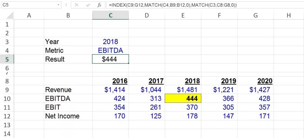
• Let’s suppose you have a simple table as shown in the picture below, and you want to retrieve the 2018 EBITDA based on the inputs of cells C3 and C4.
• Cell C5 should return the number 444, but instead is returning a #N/A error.

• To investigate where the error is originating, press F2 on cell C5 to enter “Edit” mode.
• The formula in cell C5 is displayed and is using an INDEX-MATCH-MATCH formula to retrieve the desired metric within the desired year.  The desired value is in Row 2, Column 3 of the INDEX array.

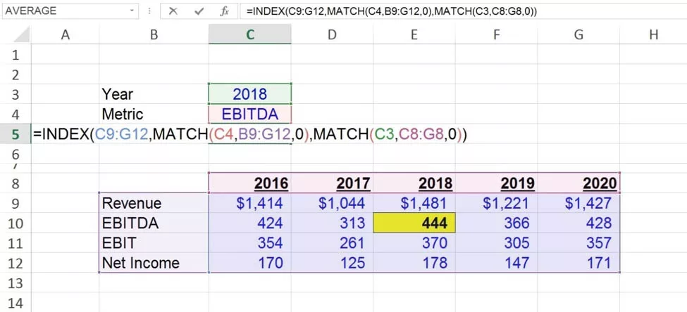
• Highlight the part of the formula that says MATCH(C3,C8:G8,0).

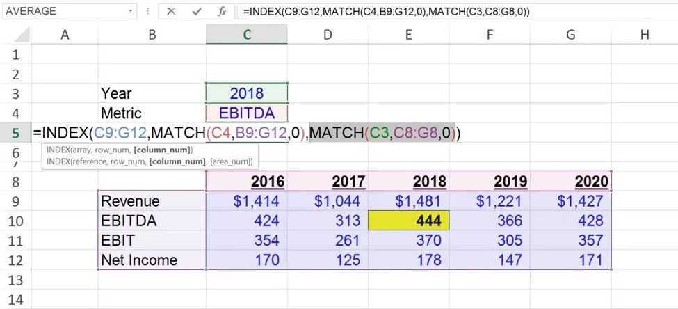
• Once highlighted, press F9. This should return the value 3, which it does.

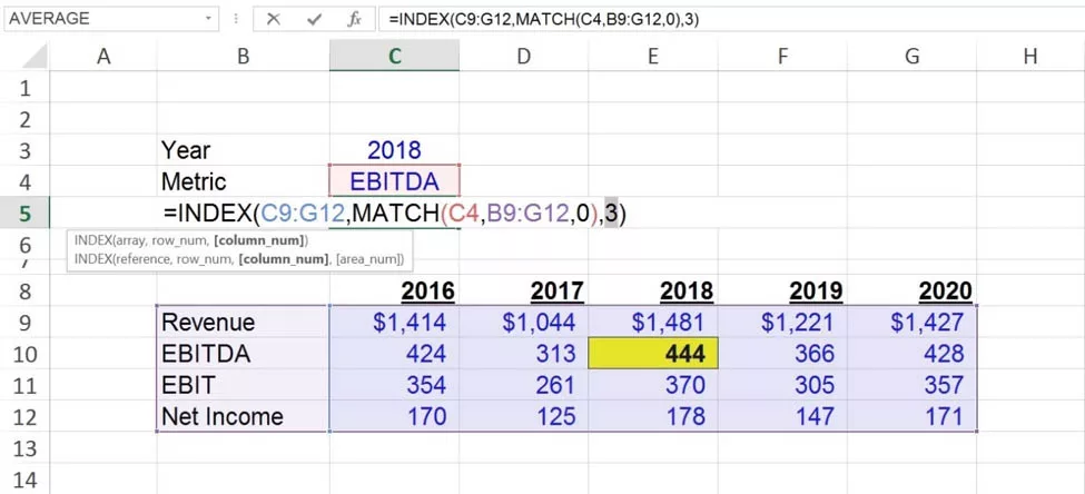
• Since this part of the formula did not produce an error, the same process can be applied to the next part of the formula.
• Highlight the part of the formula that says MATCH(C4,B9:G12,0).

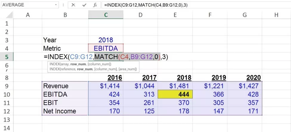
• Once highlighted, press F9. This should return the value 2, but instead returns the #N/A error.

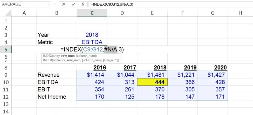
• Press the Escape key to exit “Edit” mode and return the cell back to its original formula.

• Now that the part of the formula that contained the #N/A error has been found, that part of the formula can be edited.
• To edit the formula, press F2 on cell C5 to enter “Edit” mode.
• Change MATCH(C4,B9:G12,0) to MATCH(C4,B9:B12,0) because the MATCH array should only include the column where the desired metric is found.
• Press the Enter key and cell C5 will update to display the number 444, which is the correct value.