Data Tables Part II – Building an Excel Data Table Across Worksheets
This article will dive into more detail on one of the particular issues we identified within a previous resource, which is that Excel’s data table must be on the same worksheet as the original inputs being sensitized. Part I can be found here.
Our example included a simple calculation of 2019 EBITDA and a Data Table to assess what the resulting EBITDA would be under a range of revenue growth and EBITDA margin assumptions. We connected the data table and obtained results that worked as expected.

But a common issue when building more complex models is the desire to create a separate Outputs Sheet that includes a number of key summary tables or charts in one place, rather than spread throughout a model. In the previous example, the Data Table we created belongs on an Output Sheet rather than in the body of the model.
Our first instinct is to setup the Data Table on the Output Sheet and then link back to the Calculation Sheet for our Row Input and Column Input cells in the dialog box.
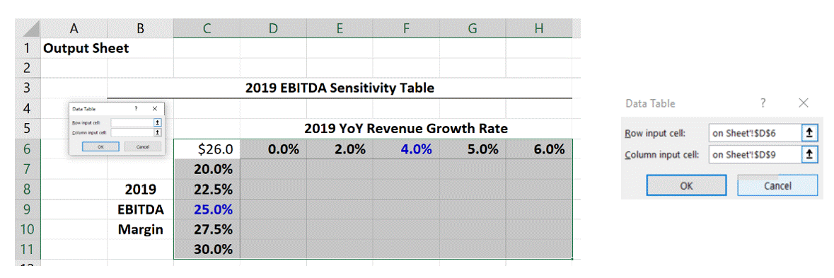
Excel will allow you to enter references to the Calculation sheet in the dialog box. But when you click OK, you will get an error message stating “Input cell reference not valid”: a classic, unclear Excel error message. In this instance, Excel is telling us that we cannot have the input cell references on a different sheet from the Data Table. But my client really wants a separate Output Sheet; what is an analyst to do?
Linking Two Tables Across Sheets
Rather than rebuilding the data table on the new Output Sheet tab, we can simply create a “dummy” table that links back to the “live” table on the Calculation Sheet. In the example below, we can see that all of the cells in the table (including the row and column headings) are linked back to the “live” data table on the Calculation Sheet.
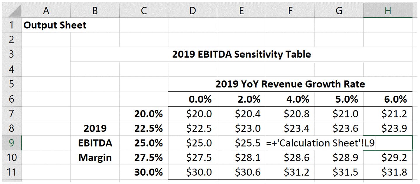
This approach works visually and creates a centralized location with key outputs. And since we’ve linked the titles and growth rates and margins (always do this!) the tables should match. Leaving the “live table” embedded within the Calculation Sheet does come with downsides, though:
- What if we wanted to add another line or column on the Calculation Sheet in a spot that would affect the “live table” (i.e. we want to add a new row between EBITDA and Margin in our example)? This would cause an error (“Can’t change part of a data table”). To solve this, we would need to delete the data in the “live table”, add the row, recreate the data table and re-link the “dummy table” on the Output Sheet. This is inefficient and prone to error or omission.
- This approach tempts model builders to hide the “live table,” either by moving it well off to the right side of the model where nobody can see it or by changing all the text white and deleting all borders. This practice is dangerous. It is prone to unintentional deletion (you can’t protect what you can’t see) and it makes a model challenging to review.
Due to these downsides, the Two Linked Tables approach is less than optimal. Luckily there is another approach.
“Dummy” Input Cells
Our original error message stems from the input cell being on a different sheet. What if we could have an input cell on the Calculation Sheet AND the Output Sheet at the same time? With some simple IF logic, we can do just that.
-
Create dummy input cells
- Create two “dummy input cells” on the Output Sheet that the Data Table can refer to. Notice that we are clearly labeling these as dummy cells that must remain blank. If this is a model with many users, we recommend protecting these cells to avoid inadvertent data entry by unsuspecting users (protected ranges are a topic for another newsletter).
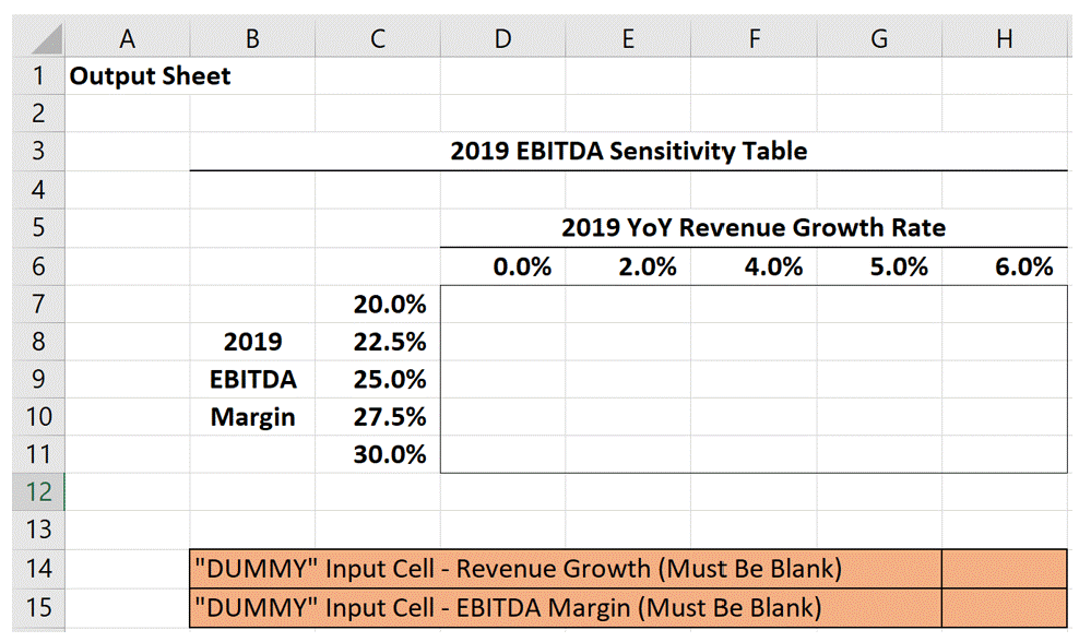
- Create two “dummy input cells” on the Output Sheet that the Data Table can refer to. Notice that we are clearly labeling these as dummy cells that must remain blank. If this is a model with many users, we recommend protecting these cells to avoid inadvertent data entry by unsuspecting users (protected ranges are a topic for another newsletter).
-
Cut and move the input cell
- In a real model, there is a high likelihood that multiple locations in the model will refer to one input cell. For that reason, you should cut and paste the old input cells to a new location so the other references throughout the model will continue to reference that cell.
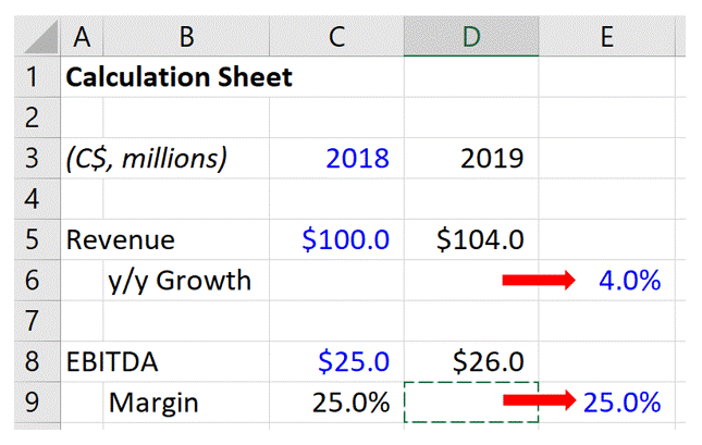
- In a real model, there is a high likelihood that multiple locations in the model will refer to one input cell. For that reason, you should cut and paste the old input cells to a new location so the other references throughout the model will continue to reference that cell.
-
Copy and paste the input value back to the original location
- We still want users to input their Revenue Growth and Margin Assumptions in column D, so we copy and paste the values back to their original location. This is where users will enter the input value for the model going forward.
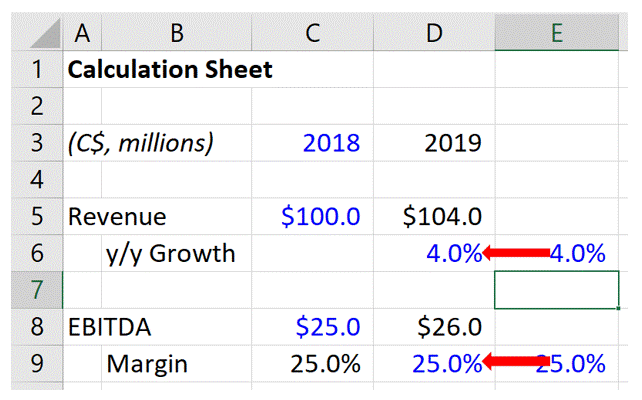
- We still want users to input their Revenue Growth and Margin Assumptions in column D, so we copy and paste the values back to their original location. This is where users will enter the input value for the model going forward.
-
Add the if logic to allow the data table to change the input
- Replace the contents of the cells in column E with the following formulas:For Revenue Growth (Cell E6):
=IF(‘Output Sheet’!H14=””,’Calculation Sheet’!D6,’Output Sheet’!H14)
For EBITDA Margin (Cell E9):
=IF(‘Output Sheet’!H15=””,’Calculation Sheet’!D9,’Output Sheet’!H15)
- Replace the contents of the cells in column E with the following formulas:For Revenue Growth (Cell E6):
-
Format & protect the new input cells
- Similar to the “Dummy Inputs” on the Output Sheet, we recommend labelling and/or protecting these new cells (E6 & E9 on the Calculation Sheet) to avoid inadvertent data entry.
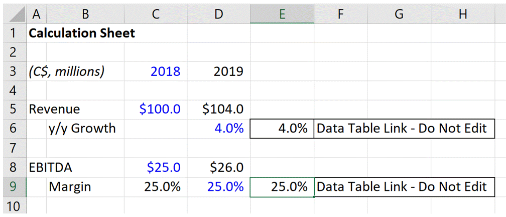
- Similar to the “Dummy Inputs” on the Output Sheet, we recommend labelling and/or protecting these new cells (E6 & E9 on the Calculation Sheet) to avoid inadvertent data entry.
-
Connect your Data Table on the Output Sheet.
- The Data Table on the output sheet can now be connected as usual, with the row input cell referring to the “Dummy” Revenue input cell and the column input cell referring to the “Dummy” Margin input cell.
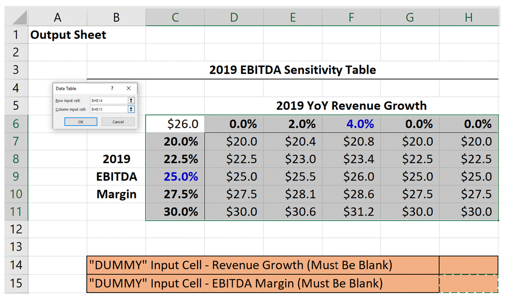
- The Data Table on the output sheet can now be connected as usual, with the row input cell referring to the “Dummy” Revenue input cell and the column input cell referring to the “Dummy” Margin input cell.
Now we have a live Data Table on your output page that is indirectly linked to input cells on another tab, eliminating data tables from the body of your model. This works because when the Data Table runs through its sensitivities, it places each Data Table combination in the Dummy Input Cells (the Data Table can ignore protection on those cells). When it does this, the IF statement on the Calculation Sheet sees that there is a value in the dummy cell and uses the value for calculations. When the Data Table is finished running, the cell returns to blank and the IF statements reverts to using the hardcoded input in column D on the Calculation Sheet.
If you enjoyed reading this and want to improve your skills further, then try our Excel Best Practices Self-Study Course. You can also browse our other range of Self-Study Courses here.
Training The Street also offers a more advanced In-Person/Virtual Public Course called, Applied Excel. Where you can gain the skills needed for parsing, analyzing, and presenting information from large data sets.
