
Dynamic Hyperlink in Excel: How to Use the HYPERLINK Function
Navigation breaks are one of the more annoying problems in financial models. You build a clean table of contents, link each section to the right row, and then someone inserts a few rows for a new assumption block. Suddenly every hyperlink points somewhere wrong. The links haven’t changed. The model has.
Static hyperlinks work by storing a fixed cell address. Move the target and the link becomes stale. This is easy to overlook during model review and genuinely frustrating to debug after the fact. The fix isn’t complicated, but it does require knowing which tool to use.
There are two approaches worth knowing: defined names and the Excel HYPERLINK function. Both solve the same root problem. Understanding when to reach for each one is the practical skill.
Why Static Hyperlinks Break
When you insert a hyperlink in Excel using Ctrl+K and select “Place in This Document,” Excel records the destination as a cell address, something like Sheet1!A45. That address is hardcoded. If you insert 10 rows above row 45, your target content is now at row 55, but the hyperlink still says 45.
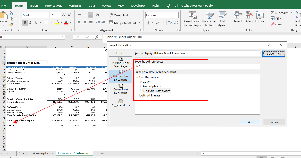
This matters most in large models with navigation menus, where analysts jump between an assumptions tab, output schedules, and supporting calculations. A broken link wastes time. In a client-facing model, it looks sloppy.
The underlying issue is that Excel’s default hyperlink behavior treats cell addresses as fixed coordinates, not as references that update dynamically. The solution is to give Excel something more stable to point to.
Solution 1: Defined Names
A defined name is exactly what it sounds like: a label you assign to a cell or range. Instead of referencing cell A45, you reference “DCF_Output” or “AssumptionsTop.” Excel always knows where that named range lives, regardless of what happens to the row structure around it.
- Select the target cell (where you want the hyperlink to land).
- Click the Name Box in the top-left corner of the screen, directly above column A.

- Type a name and press Enter. Names must start with a letter, underscore, or backslash. No spaces, no most punctuation.
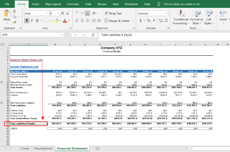
- To view or manage all names in the workbook, open the Name Manager with Ctrl+F3.
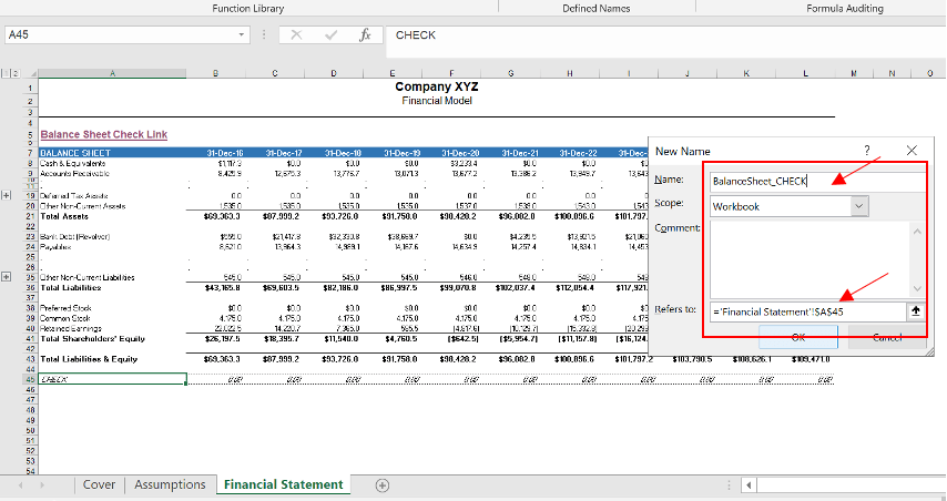
Once the name exists, insert a hyperlink with Ctrl+K, choose “Place in This Document,” and select the defined name from the list instead of typing a cell address.
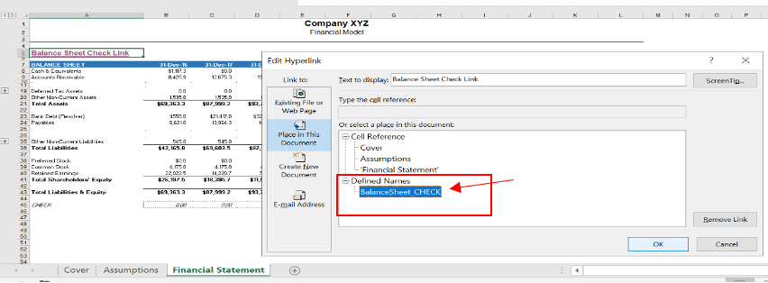
From that point on, the link follows the named range wherever it goes.
There’s a secondary benefit here. Because the link targets a name rather than a cell-plus-sheet address, you can copy or cut the hyperlink cell to a different worksheet and the reference stays intact. That’s useful when you’re building a navigation menu that needs to work from multiple tabs.
Solution 2: The Excel HYPERLINK Function
The HYPERLINK function takes a formula-based approach to the same problem.

=HYPERLINK(link_location, [friendly_name])The link_location is the destination. The optional friendly_name is the display text shown in the cell. If you skip the friendly name, Excel shows the full link location text, which is rarely what you want.
For internal references within the same workbook, the link location needs a # prefix followed by the defined name:
=HYPERLINK("#AssumptionsTop","Return to Assumptions")The hashtag tells Excel this is an internal reference, not a path to an external file or URL. Without it, the function doesn’t know where to look and will return an error or navigate nowhere useful.
You can also concatenate the # with the name string, which is useful when building links programmatically:
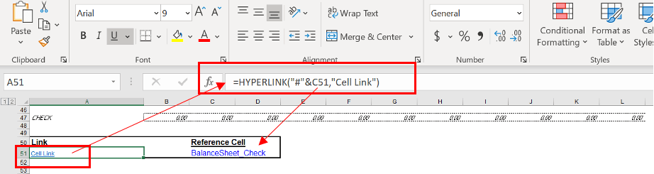
Excel’s autocomplete will surface defined names as you type, making it easy to confirm you’ve referenced the right one:
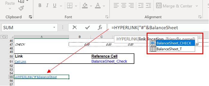
This approach works especially well when linking to Excel Table ranges, which carry their own built-in names. It also allows for more dynamic constructions: because HYPERLINK is a formula, you can build the link location programmatically, which opens up possibilities for conditional navigation or model dashboards.
Defined Names vs. HYPERLINK Function: When to Use Each
| Scenario | Recommended Approach |
|---|---|
| Simple navigation menu in a single workbook | Defined names with Ctrl+K |
| Cross-worksheet hyperlinks that need to be copied | Defined names |
| Linking to Excel Table ranges | HYPERLINK function |
| Dynamic or formula-driven link destinations | HYPERLINK function |
| Bulk navigation links built programmatically | HYPERLINK function |
Neither approach is universally better. Defined names are faster to set up for straightforward cases. The HYPERLINK function gives you more flexibility when the destination logic needs to be conditional or variable.
Putting It Together in a Financial Model
A practical use case: most well-built financial models have a cover page or menu tab that links to each section. Analysts jump from the menu to the debt schedule, then to the operating model, then to the output summary. If any of those links are static, one structural edit breaks the navigation.
The solution is to name the top cell of each destination section (something like “DebtSchedule_Top” or “OperatingModel_Top”), then build the menu using either Ctrl+K hyperlinks pointing to those names or HYPERLINK formulas. Either way, the navigation survives row insertions, column additions, and the inevitable restructuring that happens during model review.
The same principle applies to “Return to Menu” links scattered across a model. Build them with defined names or the HYPERLINK function and they’ll work from any tab, regardless of how the model evolves.
If you want to take this further, these are the two courses worth looking at.
Applied Excel
Become a Master in Excel for Finance
Advanced formula construction, model architecture, shortcuts, data manipulation, and modeling pitfalls. Covers the structural discipline that keeps complex models navigable under pressure.
Mastering Excel Bundle
Self-Paced Excel Training for Finance
Works from Excel fundamentals through to advanced modeling technique. Built for analysts who want real fluency, not just familiarity with the basics.
Includes three modules